Pre-Norm Transformer Block

每个 Transformer 块包含两个子层:多头自注意力机制和逐位置前馈网络。在原始的Transformer论文中,模型在这两个子层的外部都使用了残差连接,并在残差连接之后应用Layer Normalization。这种结构通常称为后规范化(post-norm) Transformer,因为LayerNorm被放在了子层输出的后面。

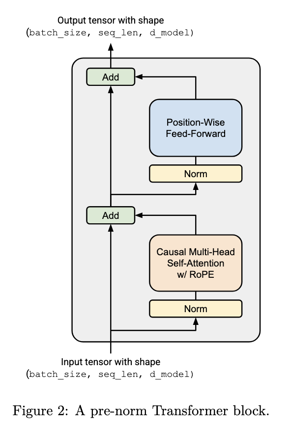
然而,许多后续研究发现,将LayerNorm从子层输出移动到子层输入(并在整个Transformer的最后再额外加一个 LayerNorm)可以提升Transformer的训练稳定性。

imagepng

这里展示了这种前规范化(pre-norm) Transformer块的结构。

在这种结构里,每个Transformer子层的输出会通过残差连接加回到子层的输入。对于pre-norm,一个常见的直觉解释是:从输入 embedding 到最终输出之间,有一条干净的、不经过归一化的“残差流(residual stream)”,被认为有助于改善梯度传播。

如今的语言模型(例如 GPT-3、LLaMA、PaLM 等)几乎都使用这种pre-norm Transformer,因此在本作业中我们也将实现这一变体。我们会依次讲解pre-norm Transformer块的各个组成部分,并按顺序实现它们。

Experiment : Root Mean Square Layer Normalization

原始的 Transformer使用Layer Normalization对激活进行归一化。我们将使用 RMSNorm(Root Mean Square Layer Normalization)来进行归一化。

给定一个激活向量aRdmodela\in\mathbb{R}^{d_{\text{model}}},RMSNorm 会按如下方式对每个激活值aia_i进行重新缩放:

RMSNorm(ai)=aiRMS(a)gi ,RMS(a)=1dmodeli=1dmodelai2+ϵRMSNorm(a_i) = \frac{a_i}{RMS(a)}g_i\ ,\\ \\ RMS(a)=\sqrt {\frac{1}{d_{model}}\sum ^{d_{model}}_{i=1}a^2_i + \epsilon}

在这里,gig_i是一个可学习的增益参数(总共有d_model个这样的参数),ϵ\epsilon是一个超参数,通常被固定为 1×1051 \times 10^{-5}

你应该将输入向上转换为torch.float32,以防在对输入进行平方时发生溢出,之后再转为原来的dtype。总之,forward方法应当看起来像这样:

1
2
3
4
5
6
7
in_dtype = x.dtype
x = x.to(torch.float32)
# Your Code here performing RMSNorm
...
result = ...
# Return the result in the original dtype
return result.to(in_dtype)

最后,在[adapters.run_rmsnorm]中实现你的功能,并用以下的语句测试:

1
uv run pytest -k test_rmsnorm

看完上面的要求先创建文件transformer/RMSNorm.py,然后写模板:

1
2
3
4
5
6
7
8
9
10
11
12
13
14
15
16
17
18
19
20
21
22
23
24
25
26
import torch
class RMSNorm(torch.nn.Module):
def __init__(self, d_model: int, eps: float = 1e-5, device=None, dtype=None):
"""
Construct the RMSNorm module.

Args:
d_model (int):
Hidden dimension of the model.

eps (float):
Epsilon value for numerical stability, defaults to 1e-5.

device (torch.device | None):
Device to store the parameters on.

dtype (torch.dtype | None):
Data type of the parameters.
"""
super().__init__()

def forward(self, x: torch.Tensor) -> torch.Tensor:
"""
Process an input tensor of shape (batch_size, sequence_length, d_model)
and return a tensor of the same shape.
"""

其实这个部分实现并不难,就是按功能写代码,就直接给结果了:

1
2
3
4
5
6
7
8
9
10
11
12
13
14
15
16
17
18
19
20
21
22
23
24
25
26
27
28
29
30
31
32
33
34
35
36
37
38
39
40
import torch
class RMSNorm(torch.nn.Module):
def __init__(self, d_model: int, eps: float = 1e-5, device=None, dtype=None):
"""
Construct the RMSNorm module.

Args:
d_model (int):
Hidden dimension of the model.

eps (float):
Epsilon value for numerical stability, defaults to 1e-5.

device (torch.device | None):
Device to store the parameters on.

dtype (torch.dtype | None):
Data type of the parameters.
"""
super().__init__()
self.d_model = d_model
self.eps = eps
kwargs = {'device': device, 'dtype': dtype}
# weight = 1
self.weight = torch.nn.Parameter(torch.ones(self.d_model, **kwargs))

def forward(self, x: torch.Tensor) -> torch.Tensor:
"""
Process an input tensor of shape (batch_size, sequence_length, d_model)
and return a tensor of the same shape.
"""
in_dtype = x.dtype
x_float = x.to(torch.float32)
rms = torch.sqrt(
reduce(x_float ** 2, 'b s d -> b s 1', 'mean') + self.eps
)
# Apply gain (broadcast)
result = x_float / rms * self.weight
# Return the result in the original dtype
return result.to(in_dtype)

代码都是按公式来的,按照einops书写的rms公式就是下面这句

1
2
3
rms = torch.sqrt(
reduce(x_float ** 2, 'b s d -> b s 1', 'mean') + self.eps
)

这句话表示“对输入张量x的最后一维d取平均,并把它缩成 1”。

缩成1主要是因为最后取平均后还需要进行广播用于张量相加和开方,因此仍然需要保留1维向量而不能是数字。

如果不使用einops而是使用传统派作风,那么应该写成下面这样:

1
rms = torch.sqrt(x.pow(2).mean(dim=-1, keepdim=True) + eps)

测试结果如下:

image\.png

另外一提,如果你分别使用einops和不使用einops来进行测试的话,你就会发现不使用的平均比使用的要慢一倍时间左右。


Position-Wise Feed-Forward Network

早期的transformer提出了由两层Linear中间夹一层ReLU层构成的前馈网络,内层前馈层的维数通常为输入维数的4倍。

然而,现代语言模型与这一最初的设计相比,有两个主要的变化:它们使用了另一个激活函数,并采用了门控机制。具体来说,我们将实现Llama 3和Qwen 2等LLM中采用的SwiGLU激活函数,它结合了SiLU (常被称为Swish)激活和一种称为门控线性单元( Gated Linear Unit,GLU )的门控机制。

我们也将省略线性层中有时使用的偏差项,沿用自PaLM和LLaMA以来的大多数现代LLM。

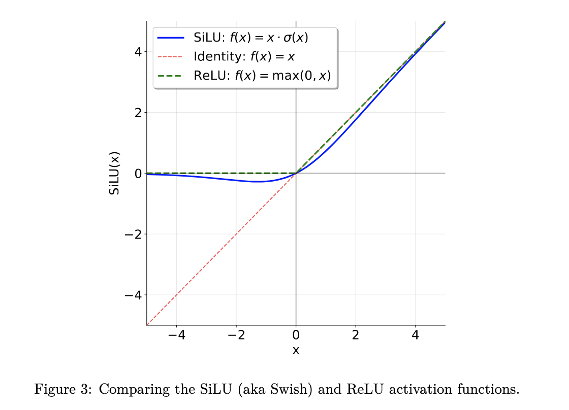
首先介绍SiLU函数,一般定义如下:

SiLU(x)=xσ(x)=x1+exSiLU(x)=x·σ(x)=\frac{x}{1+e^{-x}}

imagepng

你可以发现他和ReLU形状相似,但是在靠近0的地方是渐近的,这样可以避免梯度消失的问题。

门控线性单元GLUs最初定义为经过一个sigmoid函数的线性变换和另一个线性变换的元素级乘积,就像下面这样:

GLU(x,W1,W2)=σ(W1x)W2xGLU(x,W_1,W_2)=σ(W_1x)⊙W_2x

其中⊙表示元素级乘法。门控线性单元被建议"通过为梯度提供线性路径,同时保留非线性能力,来减少深度架构的梯度消失问题"。

将SiLU和GLU放到一起,我们就得到了SwiGLU,它将会使用在我们的前馈网络中:

FFN(x)=SwiGLU(x,W1,W2,W3)=W2(SiLU(W1x)W3x)xRdmodel,W1,W3Rdff×dmodel,W2Rdmodel×dff,dff=83dmodelFFN(x)=SwiGLU(x,W_1,W_2,W_3)=W_2(SiLU(W_1x)⊙W_3x), \\x\in \mathbb{R}^{d_{model}}, W_1,W_3\in \mathbb{R}^{d_{ff}\times d_{model}}, W_2\in \mathbb{R}^{d_{model}\times {d_{ff}}}, d_{ff}=\frac{8}{3}d_{model}

2020年Shazeer首次提出将SiLU / Swish激活与GLUs相结合,并进行了实验,实验表明SwiGLU在语言建模任务上优于ReLU和SiLU (无门控)等基线。在后面的赋值中,将对SwiGLU和SiLU进行比较。尽管我们提到了这些组件(并且论文提供了更多的佐证)的一些启发性论点,但保持一个经验主义的观点是好的:Shazeer论文中的一个著名的引述是:

“我们没有解释为什么这些架构似乎是有效的;我们把他们的成功和其他一切一样,归功于神圣的仁慈”

写这个文档的哥们到这里终于点出了机器学习的本质(

Experiment : Position-wise feed-forward network

接下来要求我们实现SwiGLU前馈网络,由SiLU激活函数和GLU组成。

注意:在这种特殊情况下,为了数值的稳定性,在实现过程中可以随意使用torch.sigmoid

另外,应该设置dff=83×dmodeld_{ff}=\frac{8}{3}\times d_{model},并同时确保内部前馈层的维度是64的倍数,以充分利用硬件。

最后,在[adapters.run_swiglu]中实现你的功能,并用以下的语句测试:

1
uv run pytest -k test_swiglu

其实这个实验和上一个一样,就是用代码单纯实现公式而已,用einops就会更加轻松。但是鉴于计算的时候维度转换问题臭名昭著,不如借这个实验来梳理一下运算过程中的维度变化。

1
2
3
4
5
# 入参维度
w1: Float[Tensor, " d_ff d_model"],
w2: Float[Tensor, " d_model d_ff"],
w3: Float[Tensor, " d_ff d_model"],
x: Float[Tensor, " ... d_model"]

输入参数weight1,weight2,weight3,x的维度如上所示。

公式W2(SiLU(W1x)W3x)W_2(SiLU(W_1x)⊙W_3x)可以分为几个部分,可以用下面几个式子分开表示:

W_1x,\\ SiLU(W_1x),\\ W_3x,\\ W_1\_W_3 = SiLU(W_1x)⊙W_3x\\ result = W_2(SiLU(W_1x)⊙W_3x)$

首先,W1x/W3xW_1x/W_3x的写法类似,他们的维度比较清晰,d_ff d_model的维度相乘后保留d_ff的维度,写法如下:

1
2
w1x = einsum(w1, x, "d_ff d_model, ... d_model -> ... d_ff")
w3x = einsum(w3, x, "d_ff d_model, ... d_model -> ... d_ff")

实际运行中他们的维度都是这样的:

1
2
3
4
5
w1:torch.Size([128, 64])
w3:torch.Size([128, 64])
x:torch.Size([4, 12, 64])
w1x:torch.Size([4, 12, 128])
w3x:torch.Size([4, 12, 128])

接下来的SiLU(W1x)SiLU(W_1x)可以直接调用torch.sigmoid()来实现,输出的维度没有变化,还是[4, 12, 128]

接下来就到了W1_W3W_1\_W_3的计算了,两个相同维度的矩阵A和B计算结果维度还是一样还是[4, 12, 128]

1
w1_w3 = einsum(self.silu(w1x), w3x, "... d_ff, ... d_ff -> ... d_ff")

最后结果的计算要求提供Float[Tensor, "... d_model"]: Output embeddings of the same shape as the input embeddings.所以最后保留的其实是d_model

1
return einsum(self.w2, w1_w3, "d_model d_ff, ... d_ff -> ... d_model")

所有的代码如下:

1
2
3
4
5
6
7
8
9
10
11
12
13
14
15
16
17
18
19
20
21
22
import torch
from einops import einsum


class SwiGLU(torch.nn.Module):
def __init__(self, d_model : int, d_ff, w1, w2, w3):
super().__init__()
self.d_model = d_model
self.d_ff = d_ff # note: d_ff = self.d_model * (8/3)
self.w1 = nn.Parameter(w1.clone()) if not isinstance(w1, nn.Parameter) else w1
self.w2 = nn.Parameter(w2.clone()) if not isinstance(w2, nn.Parameter) else w2
self.w3 = nn.Parameter(w3.clone()) if not isinstance(w3, nn.Parameter) else w3

def forward(self, x):
w1x = einsum(self.w1, x, "d_ff d_model, ... d_model -> ... d_ff")
w3x = einsum(self.w3, x, "d_ff d_model, ... d_model -> ... d_ff")
w1_w3 = einsum(self.silu(w1x), w3x, "... d_ff, ... d_ff -> ... d_ff")
return einsum(self.w2, w1_w3, "d_model d_ff, ... d_ff -> ... d_model")

@staticmethod
def silu(x):
return x * torch.sigmoid(x)

adapters.py里面的run_swiglu()函数声明这个类并调用:

1
2
3
4
5
6
7
8
9
10
11
12
13
14
15
16
17
18
19
20
21
22
23
24
25
26
27
28
29
30
31
def run_swiglu(
d_model: int,
d_ff: int,
w1_weight: Float[Tensor, " d_ff d_model"],
w2_weight: Float[Tensor, " d_model d_ff"],
w3_weight: Float[Tensor, " d_ff d_model"],
in_features: Float[Tensor, " ... d_model"],
) -> Float[Tensor, " ... d_model"]:
"""Given the weights of a SwiGLU network, return
the output of your implementation with these weights.

Args:
d_model (int): Dimensionality of the feedforward input and output.
d_ff (int): Dimensionality of the up-project happening internally to your swiglu.
w1_weight (Float[Tensor, "d_ff d_model"]): Stored weights for W1
w2_weight (Float[Tensor, "d_model d_ff"]): Stored weights for W2
w3_weight (Float[Tensor, "d_ff d_model"]): Stored weights for W3
in_features (Float[Tensor, "... d_model"]): Input embeddings to the feed-forward layer.

Returns:
Float[Tensor, "... d_model"]: Output embeddings of the same shape as the input embeddings.
"""
# Example:
# If your state dict keys match, you can use `load_state_dict()`
# swiglu.load_state_dict(weights)
# You can also manually assign the weights
# swiglu.w1.weight.data = w1_weight
# swiglu.w2.weight.data = w2_weight
# swiglu.w3.weight.data = w3_weight
module = SwiGLU(d_model, d_ff, w1_weight, w2_weight, w3_weight)
return module.forward(in_features)

测试结果如下:

image\.png

Relative Positional Embeddings

为了将编码的位置信息注入到模型中,我们将实现**旋转位置嵌入(Rotary Position Embeddings,RoPE)。**不同于传统的绝对位置编码(sin/cos 直接加到 token embeddings 上),RoPE不改变embedding本身,而是在注意力计算中对Q和K引入与位置相关的旋转,这样做具有推理快、可外推、数学自然、实现简单的优点。

对于一个位于位置ii的要查询的tokenq(i)=Wqx(i)Rdq^{(i)}=W_qx^{(i)}\in \mathbb{R}^d

我们将会对它使用一个成对旋转矩阵RiR_i,得到q(i)=Riq(i)=RiWqx(i)q'^{(i)} = R^iq^{(i)}=R^i W_q x^{(i)}。在这里,RiR^i会将嵌入的成对元素q2k1:2k(i)q^{(i)}_{2k-1:2k}作为2D向量来旋转θi,k=iΘ(2k2)/d\theta_{i,k}=\frac{i}{\Theta^{(2k-2)/d}}的角度,其中k{1,...,d/2},Θ为常数k\in\{ 1,...,d/2\},\Theta为常数

因此,我们可以将RiR_i视作一个大小为d×dd\times d的对角矩阵,由小块RkiR^i_k组成,其中

R^i_k= \begin{bmatrix} cos(\theta_{i,k}) & -sin(\theta_{i,k}) \\ sin(\theta_{i,k}) & cos(\theta_{i,k}) \end{bmatrix},\\ k\in\{1,...,d/2\}​$

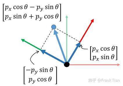
这个矩阵从数学意义上来说其实就是将每一对维度(2k−1, 2k)视为一个二维平面上的点(px,py),并根据token位置i按不同的角度θi,k\theta_{i,k} 逆时针旋转。就像下面这图一样:

imagepng

将各个位置上的token综合起来,我们就获得了完整的旋转矩阵

Ri=[R1i00...00R2i0...000R3i...0000...Rd/2i]R^i=\begin{bmatrix} R^i_1 & 0 & 0 & ... & 0 \\ 0 & R^i_2 & 0 & ... & 0 \\ 0 & 0 & R^i_3 & ... & 0 \\ \vdots & \vdots & \vdots & \ddots &\vdots \\ 0 & 0 & 0 & ... & R^i_{d/2} \end{bmatrix}

其中的0表示 2 × 2 的零矩阵。虽然我们可以构造完整的 d × d 旋转矩阵,但更好的做法是利用该矩阵的结构特性来更高效地实现这个变换。因为我们只关心序列中token之间的相对旋转,所以我们可以在不同层以及不同 batch 之间复用计算得到的cos(θi,k)cos(θ_{i,k})sin(θi,k)sin(θ_{i,k})的值。

如果你想进一步优化,可以使用一个被所有层共享的单一 RoPE 模块,并在初始化阶段通过self.register_buffer(persistent=False)创建一个预计算好的大小为2d的 sin/cos 缓冲区,而不是使用nn.Parameter(因为我们不希望去学习这些固定的正弦和余弦值)。我们对q(i)q^{(i)}所做的同样旋转,也需要对k(j)k^{(j)}做一次,按对应的RjR^j进行旋转。

注意,这一层是没有可学习参数的。

Experiment : RoPE

这个实验要求实现一个RotaryPositionalEmbedding类,能够对输入张量进行RoPE变换。

adapters.run_rope中实现功能并使用下列语句启动测试:

1
uv run pytest -k test_rope

我们创建文件transformer/RoPE.py,然后输入课程推荐的模版:

1
2
3
4
5
6
7
8
9
10
11
12
13
14
15
16
17
18
19
20
21
22
23
24
25
26

def __**init__**(self, theta: float, d_k: int, max_seq_len: int, device=None):
"""
Construct the RoPE module and create buffers if needed.
Args:
theta (float): Θ value for the RoPE.
d_k (int): Dimension of query and key vectors.
max_seq_len (int): Maximum sequence length that will be inputted.
device (torch.device | None): Device to store the buffer on.
"""

def forward(self, x: torch.Tensor, token_positions: torch.Tensor) -> torch.Tensor:
"""
Process an input tensor of shape (..., seq_len, d_k) and return a tensor of the same shape.
Note:
- x can have an arbitrary number of batch dimensions.
- token_positions is a tensor of shape (..., seq_len) specifying the token positions of x along the sequence dimension.
- Use the token positions to slice your (possibly precomputed) cos and sin tensors along the sequence dimension.

Args:
x (torch.Tensor): Input tensor.
token_positions (torch.Tensor): Tensor containing token positions along the sequence dimension.

Returns:
torch.Tensor: Output tensor of the same shape as x.
"""

首先确定我们首先要做的是什么:应该是创建一个与输入张量x和位置信息token_positions无关的旋转变换矩阵RiR^i。因为后续还需要对k(j)k^{(j)}重复做一次旋转操作,所以这个矩阵的信息应当长期保存。

考虑到这个矩阵实际上是个块对角矩阵,也就是说上文公式中每个元素实际上都是一个大小为2×22\times 2的小矩阵(这个小矩阵就是上文里面sin cos公式的那一个),其他位置都是零矩阵,于是实际上我们只需要使用 2*2*d/2 = 2d大小的线性空间就可以存储下整个矩阵的信息。

然而,我们实际上并不会存储下这个矩阵,更普遍的做法是使用q2k1:2k(i)q^{(i)}_{2k-1:2k}来与小旋转矩阵相乘,那么实际上就是[x[: , 2i - 1],x[: , 2i]]与矩阵 [cos(θi,k)sin(θi,k)sin(θi,k)cos(θi,k)]\begin{bmatrix} cos(\theta_{i,k}) & -sin(\theta_{i,k}) \\ sin(\theta_{i,k}) & cos(\theta_{i,k}) \end{bmatrix}相乘。把x的奇数项记成x_odd,偶数项记成x_even,结果就表达为[x_odd * cos(θ) + x_even * sin(θ) , x_even * cos(θ) - x_odd * sin(θ)]。也就是说,可以将x分为奇数和偶数两个序列进行计算,再将结果进行合并即可。这样我们只需要分别保存sin和cos提前计算的值。

1
2
3
4
5
6
7
8
9
10
11
12
13
14
15
16
17
18
19
20
21
22
23
24
25
26
27
28
29
30
31
32
33
34
35
36
37
38
39
40
41
42
43
44
45
46
47
48
49
50
51
52
53
54
55
56
57
from torch import nn
import torch


class RotaryPositionalEmbedding(nn.Module):

def __init__(self, theta: float, d_k: int, max_seq_len: int, device=None):
"""
Construct the RoPE module and create buffers if needed.
Args:
theta (float): Θ value for the RoPE.
d_k (int): Dimension of query and key vectors.
max_seq_len (int): Maximum sequence length that will be inputted.
device (torch.device | None): Device to store the buffer on.
"""
super().__init__()
if d_k % 2 != 0:
raise ValueError("d_k must be even for RoPE")
self.theta = theta
self.d_k = d_k
self.max_seq_len = max_seq_len
# 1 / *Θ^((2k - 2) / d)*
frequency = 1.0 / (theta ** (torch.arange(0, d_k, 2).float() / d_k))
# position = [0,1,...,i]
position = torch.arange(max_seq_len, device=device)
rotate_theta = torch.outer(position, frequency)

self.register_buffer('sin_register', rotate_theta.sin(), persistent=False)
self.register_buffer('cos_register', rotate_theta.cos(), persistent=False)

def forward(self, x: torch.Tensor, token_positions: torch.Tensor) -> torch.Tensor:
"""
Process an input tensor of shape (..., seq_len, d_k) and return a tensor of the same shape.
Note:
- x can have an arbitrary number of batch dimensions.
- token_positions is a tensor of shape (..., seq_len) specifying the token positions of x along the sequence dimension.
- Use the token positions to slice your (possibly precomputed) cos and sin tensors along the sequence dimension.

Args:
x (torch.Tensor): Input tensor.
token_positions (torch.Tensor): Tensor containing token positions along the sequence dimension.

Returns:
torch.Tensor: Output tensor of the same shape as x.
"""
sin_theta = self.sin_register[token_positions]
cos_theta = self.cos_register[token_positions]

x_even = x[... , 0::2]
x_odd = x[... , 1::2]
# x_odd * cos(θ) + x_even * sin(θ) , x_even * cos(θ) - x_odd * sin(θ)
x_even_calc = x_even * cos_theta - x_odd * sin_theta
x_odd_calc = x_odd * cos_theta + x_even * sin_theta

calc = torch.stack([x_even_calc, x_odd_calc], dim=-1)
result = calc.flatten(-2)
return result

以上的代码借鉴自和鲸社区,在此感谢~

作者: 天海一直在AI

来源: 斯坦福大学CS336从零实现大语言模型课程作业复现——Transformer

__init__()中就实现了对于全部token位置的矩阵sin和cos值的计算,并将其保存在sin_registercos_register中。而在forward()中会根据传入的token_positions从缓存中直接取出对应的sin和cos值。再将x分奇偶按公式相乘,最后还原为原始矩阵形状就能完成计算。

做这个实验的过程中,其实是最后的还原阶段最令人疑惑:stack的结果是怎样的?flatten的作用又是什么?

cat & stack & flatten

先来谈谈stack,其实还有一个和他作用很接近的函数cat

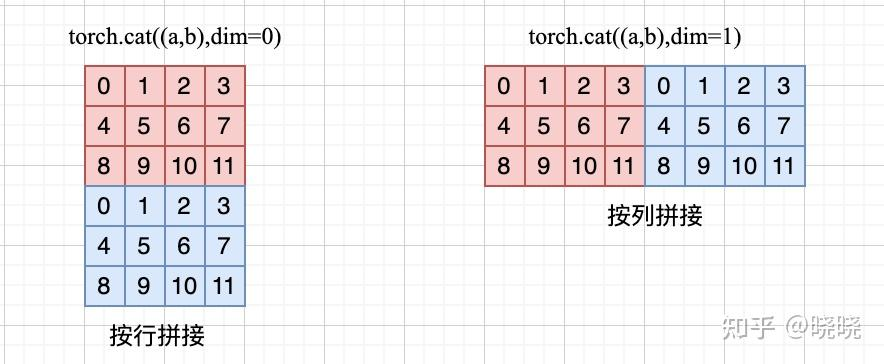
  • torch.cat可以理解成“拼接”,可以按行拼接,也可以按列拼接。操作后得到的张量维度不会增加。要求用来拼接的张量形状匹配(但不要求张量形状完全一致,只要求非拼接维度一致)。

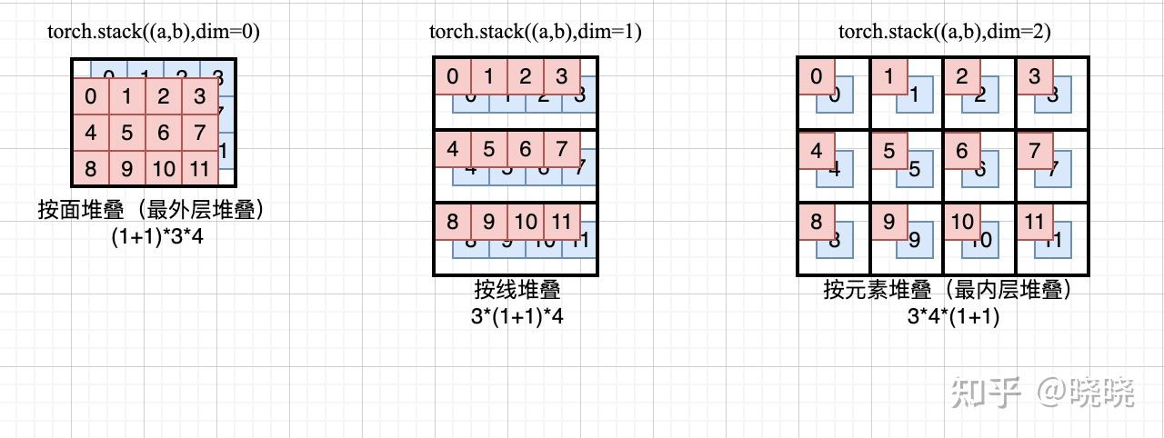
  • torch.stack可以理解成“堆叠”,操作后得到的张量会增加一维。用来堆叠的张量形状必须完全一致。

为了方便理解,不妨用一个实际例子来说:

1
2
3
4
5
6
7
8
9
10
11
12
13
import torch
import numpy as np
a = torch.from_numpy(np.arange(0,12).reshape(3, 4))
b = torch.from_numpy(np.arange(0,12).reshape(3, 4))
print(f'a={a}')
print(f'b={b}')

a=tensor([[ 0, 1, 2, 3],
[ 4, 5, 6, 7],
[ 8, 9, 10, 11]])
b=tensor([[ 0, 1, 2, 3],
[ 4, 5, 6, 7],
[ 8, 9, 10, 11]])

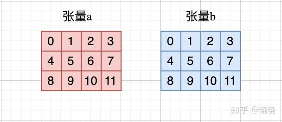
上面的代码创建了两个相同内容的3行4列的矩阵A和B。

imagepng

接下来用cat将这两个矩阵按行/按列拼接。

1
2
3
4
5
6
7
8
9
10
11
12
13
14
15
16
17
18
19
20
# torch.cat可以理解成拼接,dim=0表示按行拼接,dim=1表示按列拼接,不增加维度
c0 = torch.cat((a, b), dim=0)
print(f'c0.shape:{c0.shape}\nc0={c0}')

c0.shape:torch.Size([6, 4])
c0=tensor([[ 0, 1, 2, 3],
[ 4, 5, 6, 7],
[ 8, 9, 10, 11],
[ 0, 1, 2, 3],
[ 4, 5, 6, 7],
[ 8, 9, 10, 11]])


c1=torch.cat((a,b),dim=1)
print(f'c1.shape:{c1.shape}\nc1={c1}')

c1.shape:torch.Size([3, 8])
c1=tensor([[ 0, 1, 2, 3, 0, 1, 2, 3],
[ 4, 5, 6, 7, 4, 5, 6, 7],
[ 8, 9, 10, 11, 8, 9, 10, 11]])

很好理解,按行拼接结果就是(3 + 3, 4) = (6, 4)。按列拼接的结果则是(3, 4 + 4) = (3, 8)。

显然,按行拼接要求两个张量的列数必须一致,按列拼接要求两个张量的行数必须一致,即非拼接维度的形状必须匹配

imagepng

接下来就到了stack。首先要区分它和cat的最大区别,就是cat的结果不会增加维数,而stack会。

1
2
3
4
5
6
7
8
9
10
11
12
13
14
15
16
17
18
19
20
21
22
23
24
25
26
27
28
29
30
31
32
33
34
35
36
37
38
39
s0=torch.stack((a,b),dim=0)
print(f's0.shape:{s0.shape}\ns0={s0}')
s1=torch.stack((a,b),dim=1)
print(f's1.shape:{s1.shape}\ns1={s1}')
s2=torch.stack((a,b),dim=2)
print(f's2.shape:{s2.shape}\ns2={s2}')

s0.shape:torch.Size([2, 3, 4])
s0=tensor([[[ 0, 1, 2, 3],
[ 4, 5, 6, 7],
[ 8, 9, 10, 11]],

[[ 0, 1, 2, 3],
[ 4, 5, 6, 7],
[ 8, 9, 10, 11]]])
s1.shape:torch.Size([3, 2, 4])
s1=tensor([[[ 0, 1, 2, 3],
[ 0, 1, 2, 3]],

[[ 4, 5, 6, 7],
[ 4, 5, 6, 7]],

[[ 8, 9, 10, 11],
[ 8, 9, 10, 11]]])
s2.shape:torch.Size([3, 4, 2])
s2=tensor([[[ 0, 0],
[ 1, 1],
[ 2, 2],
[ 3, 3]],

[[ 4, 4],
[ 5, 5],
[ 6, 6],
[ 7, 7]],

[[ 8, 8],
[ 9, 9],
[10, 10],
[11, 11]]])

由于torch默认tensor的维度是**Row-major (C-order),靠右的维度变化快,靠左的维度变化慢。或者说右边的维度总是被左边维度包含着的,越右边的维度就越内层,越先展开,**因此stack的参数dim表示要在哪里创建一个新维度并进行合并。如下图所示,如果是dim = 0,那么表示在(3, 4)的最左边加入一维以合并,得到的结果就是按面堆叠(1 + 1, 3, 4)。如果是dim = 1,那么就在中间加入一维,结果就是行优先的按线堆叠(3, 1 + 1, 4)。如果是dim = 2那么就在最内层堆叠,即按元素堆叠(3, 4, 1 + 1)。

imagepng

以上内容参考图解torch.cat()和torch.stack()的区别 ,在此感谢~

flatten表示的是“展平”操作,可以看成是把一个张量的某几个维度的元素按照次序一个个依次摆放到一条直线上,也就是把高维向量展平到一维向量上。

一般来说flatten携带两个参数(start_dim, end_dim),表示要展平的维度范围[start_dim, end_dim](注意左右都闭),默认start_dim = 0end_dim = -1

imagepng

比如下面这个例子:

1
2
3
4
5
6
7
8
9
10
11
12
13
14
import torch
import numpy as np
a = torch.arange(24).reshape(2,3,4)
print (f'a.shape:{a.shape}\na={a}')

f0 = torch.flatten(a, start_dim=0)
print(f'f0.shape:{f0.shape}\nf0={f0}')
f1 = torch.flatten(a, start_dim=1)
print(f'f1.shape:{f1.shape}\nf1={f1}')
f2 = torch.flatten(a, start_dim=2)
print(f'f2.shape:{f2.shape}\nf2={f2}')

f1_2 = torch.flatten(a, end_dim=-2)
print(f'f1_2.shape:{f1_2.shape}\nf1_2={f1_2}')
1
2
3
4
5
6
7
8
9
10
11
12
13
14
15
16
17
18
19
20
21
22
23
24
25
26
27
28
29
30
31
32
33
a.shape:torch.Size([2, 3, 4])
a=tensor([[[ 0, 1, 2, 3],
[ 4, 5, 6, 7],
[ 8, 9, 10, 11]],

[[12, 13, 14, 15],
[16, 17, 18, 19],
[20, 21, 22, 23]]])
# 0~2
f0.shape:torch.Size([24])
f0=tensor([ 0, 1, 2, 3, 4, 5, 6, 7, 8, 9, 10, 11, 12, 13, 14, 15, 16, 17,
18, 19, 20, 21, 22, 23])
# 1~2
f1.shape:torch.Size([2, 12])
f1=tensor([[ 0, 1, 2, 3, 4, 5, 6, 7, 8, 9, 10, 11],
[12, 13, 14, 15, 16, 17, 18, 19, 20, 21, 22, 23]])
# 2~2
f2.shape:torch.Size([2, 3, 4])
f2=tensor([[[ 0, 1, 2, 3],
[ 4, 5, 6, 7],
[ 8, 9, 10, 11]],

[[12, 13, 14, 15],
[16, 17, 18, 19],
[20, 21, 22, 23]]])
# 0~1
f1_2.shape:torch.Size([6, 4])
f1_2=tensor([[ 0, 1, 2, 3],
[ 4, 5, 6, 7],
[ 8, 9, 10, 11],
[12, 13, 14, 15],
[16, 17, 18, 19],
[20, 21, 22, 23]])

了解了几个函数的用法后回到RoPE上来,这两句话发挥的作用就一目了然了(吗?

1
2
calc = torch.stack([x_even_calc, x_odd_calc], dim=-1)
result = calc.flatten(-2)

首先,将x偶数和奇数顺序的元素序列通过stack堆叠在一起,由于dim = -1,因此是在最内层堆叠,也就是元素堆叠,形状应该是(..., seq_len, d_k // 2, 1 + 1)。然后使用flatten(-2)[:-2]的维度展平,也就是将最后两个维度展平为一维,结果形状就是(..., seq_len, d_k)。并且由于都是行优先策略进行的堆叠和展平,因此最后的tensor元素顺序也是按行顺序来的,与一开始奇偶分开的顺序是一致的。

如果你不想考虑这么多的话,可以创建一个与x大小一致的张量out,然后按位置给out赋值就行

最后测试结果如下:

imagepng